The Global Change Assessment Model (GCAM)
Short overview
The Global Change Assessment Model (GCAM) is a global integrated assessment model that represents both human and Earth system dynamics. It explores the behaviour and interactions between the energy system, agriculture and land use, the economy and climate. The role of GCAM is to bring multiple human and physical Earth systems together in one place to provide scientific insights that would not be available from the exploration of individual scientific research lines. The model components provide a faithful representation of the best current scientific understanding of underlying behaviour.
GCAM allows users to explore what-if scenarios, quantifying the implications of possible future conditions. These outputs are not predictions of the future; they are a way of analysing the potential impacts of different assumptions about future conditions. GCAM reads in external “scenario assumptions” about key drivers (e.g., population, economic activity, technology, and policies) and then assesses the implications of these assumptions on key scientific or decision-relevant outcomes (e.g., commodity prices, energy use, land use, water use, emissions, and concentrations).
It is used to explore and map the implications of uncertainty in key input assumptions and parameters into implied distributions of outputs, such as GHG emissions, energy use, energy prices, and trade patterns. Techniques include scenarios analysis, sensitivity analysis, and Monte Carlo simulations.
GCAM has been used to produce scenarios for national and international assessments ranging from the very first IPCC scenarios (Response Strategies Working Group, 1990) through the present Shared Socioeconomic Pathways (SSPs) (Calvin et al., 2017).
Key features of the GCAM model
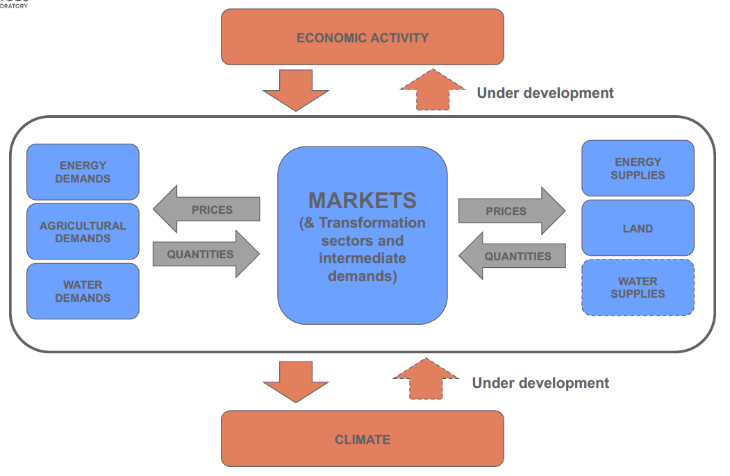
GCAM takes in a set of assumptions and then processes those assumptions to create a full scenario of prices, energy and other transformations, and commodity and other flows across regions and into the future. The energy, agriculture and land use, economy and climate systems are interconnected and interact with each other (see the figure below). The interactions between these different systems are modelled as one integrated whole.
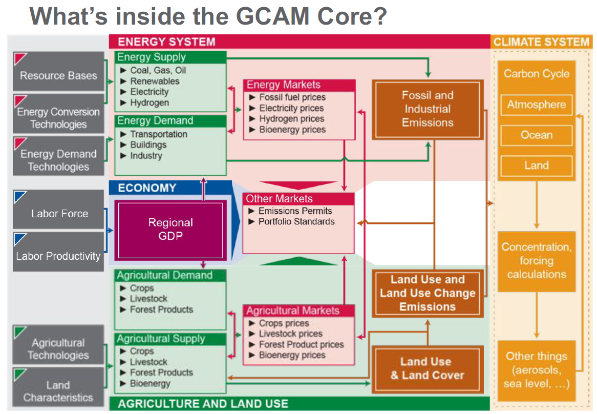
Representation of GCAM Core functioning
Geographic coverage
The GCAM core represents the entire world, but it is constructed with different levels of resolution for each of these different systems. The energy-economy system operates at 32 geopolitical regions globally , water withdrawals are tracked for 235 hydrologic basins worldwide, and to avoid overlap between geopolitical regions and hydrologic basins, agriculture and land use is calibrated for 384 regions worldwide.
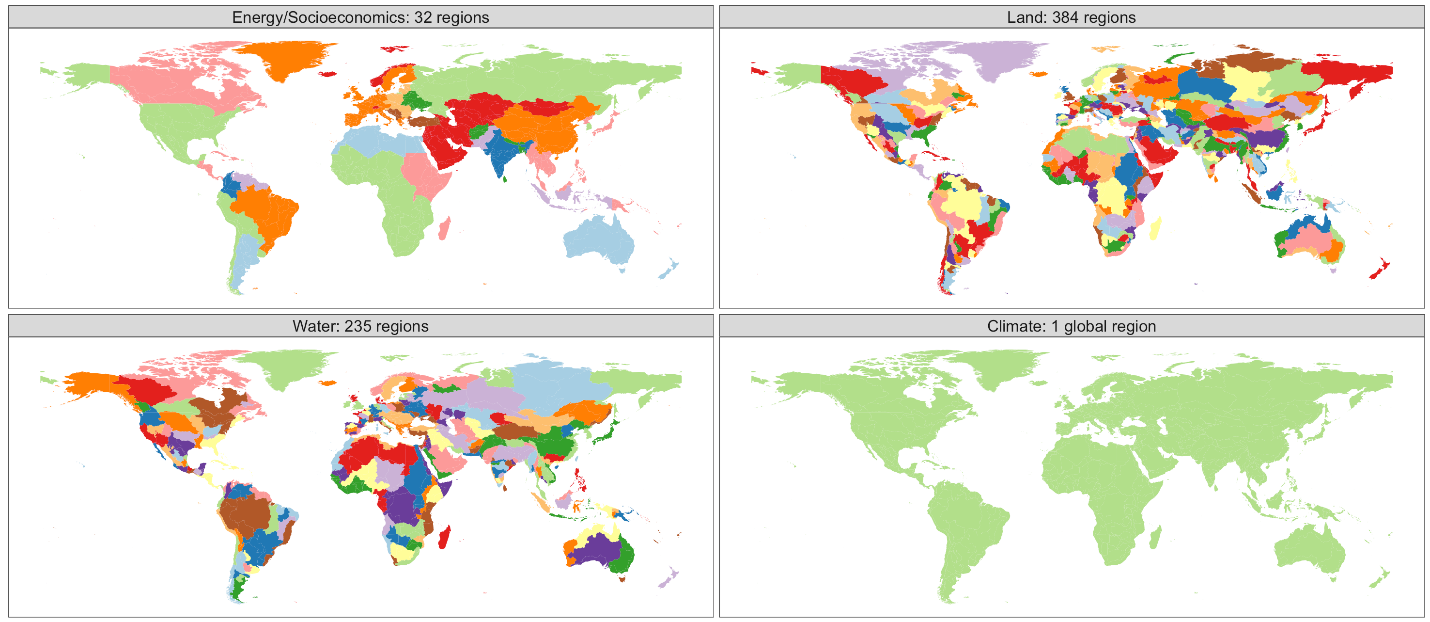
GCAM regional mapping
| Geographic region | Countries |
|---|---|
| Eastern Africa | Burundi, Comoros, Djibouti, Eritrea, Ethiopia, Kenya, Madagascar, Mauritius, Reunion, Rwanda, Sudan, Somalia, Uganda |
| Northern Africa | Algeria, Egypt, Western Sahara, Libya, Morocco, Tunisia |
| Southern Africa | Angola, Botswana, Lesotho, Mozambique, Malawi, Namibia, Swaziland, Tanzania, Zambia, Zimbabwe |
| Western Africa | Benin, Burkina Faso, Central African Republic, Cote d’Ivoire, Cameroon, Democratic Republic of the Congo, Congo, Cape Verde, Gabon, Ghana, Guinea, Gambia, Guinea-Bissau, Equatorial Guinea, Liberia, Mali, Mauritania, Niger, Nigeria, Senegal, Sierra Leone, Sao Tome and Principe, Chad, Togo |
| Argentina | Argentina |
| Australia and New Zealand | Australia, New Zealand |
| Brazil | Brazil |
| Canada | Canada |
| Central America and the Caribbean | Aruba, Anguilla, Netherlands Antilles, Antigua & Barbuda, Bahamas, Belize, Bermuda, Barbados, Costa Rica, Cuba, Cayman Islands, Dominica, Dominican Republic, Guadeloupe, Grenada, Guatemala, Honduras, Haiti, Jamaica, Saint Kitts and Nevis, Saint Lucia, Montserrat, Martinique, Nicaragua, Panama, El Salvador, Trinidad and Tobago, Saint Vincent and the Grenadines |
| Central Asia | Armenia, Azerbaijan, Georgia, Kazakhstan, Kyrgyzstan, Mongolia, Tajikistan, Turkmenistan, Uzbekistan |
| China | China |
| Colombia | Colombia |
| EU-12 | Bulgaria, Cyprus, Czech Republic, Estonia, Hungary, Lithuania, Latvia, Malta, Poland, Romania, Slovakia, Slovenia |
| EU-15 | Andorra, Austria, Belgium, Denmark, Finland, France, Germany, Greece, Greenland, Ireland, Italy, Luxembourg, Monaco, Netherlands, Portugal, Sweden, Spain, United Kingdom |
| Eastern Europe | Belarus, Moldova, Ukraine |
| European Free Trade Association | Iceland, Norway, Switzerland |
| Non-EU Europe | Albania, Bosnia and Herzegovina, Croatia, Macedonia, Montenegro, Serbia, Turkey |
| India | India |
| Indonesia | Indonesia |
| Japan | Japan |
| Mexico | Mexico |
| Middle East | United Arab Emirates, Bahrain, Iran, Iraq, Israel, Jordan, Kuwait, Lebanon, Oman, Palestine, Qatar, Saudi Arabia, Syria, Yemen |
| Pakistan | Pakistan |
| Russia | Russia |
| South Africa | South Africa |
| Northern South America | French Guiana, Guyana, Suriname, Venezuela |
| Southern South America | Bolivia, Chile, Ecuador, Peru, Paraguay, Uruguay |
| Southeast Asia | American Samoa, Brunei Darussalam, Cocos (Keeling) Islands, Cook Islands, Christmas Island, Fiji, Federated States of Micronesia, Guam, Cambodia, Kiribati, Lao Peoples Democratic Republic, Marshall Islands, Myanmar, Northern Mariana Islands, Malaysia, Mayotte, New Caledonia, Norfolk Island, Niue, Nauru, Pacific Islands Trust Territory, Pitcairn Islands, Philippines, Palau, Papua New Guinea, Democratic People’s Republic of Korea, French Polynesia, Singapore, Solomon Islands, Seychelles, Thailand, Tokelau, Timor Leste, Tonga, Tuvalu, Viet Nam, Vanuatu, Samoa |
| South Korea | South Korea |
| Taiwan | Taiwan |
| USA | United States |
Energy system detail
The structure of the energy system consists of four main elements: resource production, energy transformation, final energy carriers and end-use (see the figure below). It also tracks international trade in energy commodities. All the different elements of GCAM interact through market prices and physical flows of, for example, electricity.
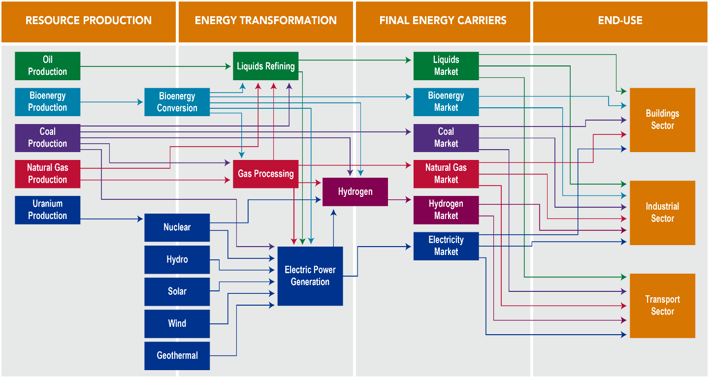
Structure of Energy system in GCAM
Land and agricultural system detail
Within each of the land regions shown in the second figure, land is categorised into approximately a dozen types based on cover and use. In GCAM, competing uses of land are nested within land nodes. Within each land node, it is generally assumed to be easier to substitute products. Among arable land types, further divisions are made for lands historically in non-commercial uses (forests and grasslands) and commercial land uses (commercial forests and croplands). Production of approximately twenty crops is currently modelled, with specific yields depending on the land region and management type (with and without irrigation, high and low fertiliser).
Climate module & emissions granularity
GCAM uses a global climate carbon-cycle climate module, Hector (Calvin et al., 2019), an open-source, object-oriented, reduced-form global climate carbon-cycle model that represents the most critical global-scale earth system processes. At every time step, emissions from GCAM are passed to Hector. Hector converts these emissions to concentrations and calculates the associated radiative forcing and the response of the climate system (e.g., temperature, carbon-fluxes, etc.).
| Gas | Sector | Gas | Sector |
|---|---|---|---|
| C02** | AgLU***, Energy | NH3 | AgLU, Energy |
| CH4 | AgLU, Energy, Industrial Processes, Urban Processes | SO2 | AgLU, Energy, Industrial Processes |
| N20 | AgLU, Energy, Industrial Processes, Urban Processes | CO | AgLU, Energy, Industrial Processes |
| SF6 | Energy, Industrial Processes | BC | AgLU, Energy |
| HFCs | Energy, Industrial Processes, Urban Processes | OC | AgLU, Energy |
| NOx | AgLU, Energy, Industrial Processes | ||
| NMVOC | AgLU, Energy, Industrial Processes, Urban Processes | ||
| C2F6 | Energy, Industrial Processes | ||
| CF4 | Industrial Processes, Urban Processes |
* Most of these gases also have positive or negative indirect effects on radiative forcing
**CO2 emissions from the AgLU sector are separate from CO2 emissions from the Energy sector. Any change in atmospheric carbon occurs as a function of anthropogenic fossil fuel and industrial emissions, land-use change emissions and the atmosphere-ocean and atmosphere-land carbon fluxes.
***AgLU = Agriculture and Land Use
Hector has a three-part main carbon cycle: a one-pool atmosphere, three-pool land, and four-pool ocean (see the figure below). The atmosphere consists of one well-mixed box. The ocean consists of four boxes, with advection and water mass exchange simulating circulation. The high-latitude surface ocean takes up carbon from the atmosphere, while the low-latitude surface ocean off-gases carbon to the atmosphere. The land consists of a user-defined number of biomes or regions for vegetation, detritus and soil. The vegetation takes up carbon from the atmosphere while the detritus and soil release carbon back into the atmosphere. The earth pool is continually debited with each time step to act as a mass balance check on the carbon system. Hector actively solves the inorganic carbon system in the surface ocean, directly calculating air– sea fluxes of carbon and ocean pH. It reproduces the global historical trends of atmospheric [CO2], radiative forcing, and surface temperatures.
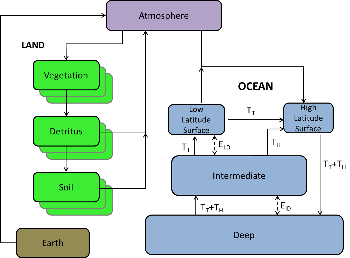
Representation of Hector’s carbon cycle, land, atmosphere, and ocean used in GCAM
Socioeconomic dimensions
Economic growth
The socioeconomic components of GCAM set the scale of economic activity and associated demands for model simulations. Assumptions about population and per capita GDP growth for each of the 32 geo-political regions together determine the GDP. Population and economic activity are used in GCAM to transfer information to other GCAM components, and are determined exogenously.
GCAM’s inputs include information on population and the rate of per capita income growth for each of the energy-economic regions. Each scenario requires assumptions about population and per capita GDP growth for future time periods, for example those of the SSPs. The macro-economic module takes both of these to produce overall GDP in each GCAM energy-economic region, where the regional GDP is calculated using a simple one-equation model:
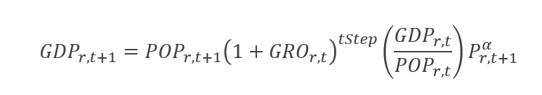
Where r stands for region, t for period, t Step = number of years in the time step (5 for GCAM), 〖GDP〗_(r,t) for GDP in region r in period t, 〖POP〗_(r,t) for population in region r in period t and 〖GRO〗_(r,t) for annual average per capita GDP growth rate in region r in period t.
Industrial sector growth
Industrial sector growth Growth in industrial sectors is based on a pre-defined GDP elasticity which decreases over time, thus assuming saturation of industrial demand with rising incomes. The values of these elasticities vary per region and between different SSPs. Apart from a GDP elasticity, industrial demand also depends on an assumed price elasticity for industrial energy use.
Transport sector growth
Per capita demand for passenger transport depends on an assumed GDP per capita elasticity and price elasticity, which means that more transport services are demanded at higher incomes and cheaper transport. However, there is also a time cost involved in transport, which increases proportionally with GDP per capita, and which is summed to the capital and energy costs of transport. This means that, at higher incomes, demand for passenger transport slowly saturates due to the price elasticity multiplied by the increasing costs of time. Also, demand shifts to faster ways of transport, for which time costs are lower. Demand for freight transport, like for industrial sectors, depends on an assumed GDP elasticity and price elasticity.
Building sector growth
Demand for energy services in residential and commercial buildings is primarily by total building floor space, which is driven by GDP per capita, and saturates at a given maximum value, defined per region. Per unit of floor space, demand for energy services increases over time depending on the relative price of the service, and the difference between the base year saturation and the defined maximum saturation for a certain service. For heating and cooling services, the maximum saturation depends on regionally explicit heating and cooling degree days.
Demand for agricultural commodities
Per capita demand for crops, animal products and forest products depend on assumed income and price elasticities. By default, price elasticities for crops and forest products are equal to 0 throughout the future, which means that these basic needs will be fulfilled, independent of commodity prices. Demand for animal products depends on the price of such products, as well as incomes, and assumptions in income elasticities vary strongly between different SSPs.
Mitigation/adaptation measures and technologies
GCAM is a technology-rich model that represents most major fossil fuel and low-carbon technologies that are envisaged to be available for at least the first half of the 21st century. By simulating the substitution of low-carbon for high-carbon technologies in response to their relative costs, as well as emissions constraints and/or carbon prices, the GCAM model simulates mitigation through a large set of different measures (see model template).
| Upstream | |
|---|---|
| Synthetic fuel production | Hydrogen production |
Coal to gas with CCS Coal to liquids with CCS Gas to liquids with CCS Biomass to liquids (with and without CCS) |
Electrolysis Coal to hydrogen with CCS Gas to hydrogen with CCS Thermal splitting (nuclear) |
| Electricity and heat | |
| Electricity generation | Heat generation |
|
Coal with CCS Gas with CCS Nuclear (fission and fusion) Hydro Biomass (with and without CCS) Geothermal Solar PV Solar CSP Wind (onshore) Marine |
Coal with CCS Gas with CCS Oil with CCS Geothermal Biomass Biomass with CCS |
| Transport | |
| Road | Rail |
|
Gas (LNG / CNG) vehicle Hybrid electric vehicles Fully electric vehicles Hydrogen fuel cell vehicles Biofuels in fuel mix |
Electric Hydrogen Efficiency |
| Air | Marine |
|
Biofuels in fuel mix |
Gas Hydrogen Biofuels Efficiency |
| Buildings | |
| Heating | Lighting |
|
Gas replacing coal / oil Biofuels Electricity Efficiency |
|
| Behaviour | Cooling |
|
Behavioural change |
Electricity |
| Process heat | CHP |
|
Gas replacing oil / coal Biomass Hydrogen Electricity |
Gas replacing oil / coal Biomass |
| Land & Animal husbandry | Behaviour |
|
Land yield maximisation Improved feeding practices |
Behavioural changes (less product demand) |
| Land Use, Land Use Change, Forestry | |
|
Afforestation Land production Biomaterials |
|
Also, certain assumption sets can be loaded for future crop yields, heating and cooling degree days, which are consistent with a certain temperature target. Through these assumptions, the model adapts to the simulated reality through the allocation of agricultural production, and building service demands.
Economic rationale and model solution
The core operating principle for GCAM is that of market equilibrium. The representative agents in the modules use information on prices and make decisions about the allocation of resources. They represent, for example, regional electricity sectors, regional refining sectors, regional energy demand sectors, and land users who have to allocate land among competing crops within any given land region. Markets are the means by which these representative agents interact with one another. Agents indicate their intended supply and/or demand for goods and services in the markets. GCAM solves for a set of market prices so that supplies and demands are balanced in all these markets across the model (see the figure below); in other words, market equilibrium is assumed to take place in each one of these markets (partial equilibrium), and not in the entire economy across all markets (general equilibrium). The GCAM solution process is the process of iterating on market prices until this equilibrium is reached. Markets exist for physical flows such as electricity or agricultural commodities, but they also can exist for other types of goods and services, for example tradable carbon permits.
As an example, in any single model period, GCAM derives a demand for natural gas starting with all of the uses to which natural gas might be put, such as passenger and freight transport, power generation, hydrogen production, heating, cooling and cooking, fertiliser production, and other industrial energy uses. Those demands depend on the external assumptions about, for example, electricity generating technology efficiencies, but also on the price of all of the commodities in the model. GCAM then calculates the amount of natural gas that suppliers would like to supply given their available technology for extracting resources and the market price. The model gathers this same information for all of the commodities and then adjusts prices so that in every market during that period supplies of everything from rice to solar power match demands.
Conceptual Schematic of the Operation of the GCAM Core
GCAM is a dynamic recursive model, meaning that decision-makers do not know the future when making a decision today, as opposed to other optimisation models, which assume that agents know the future with certainty when they make decisions. After it solves each period, the model then uses the resulting state of the world, including the consequences of decisions made in that period—such as resource depletion, capital stock retirements and installations, and changes to the landscape—and then moves to the next time step and performs the same exercise. The GCAM version used is typically operated in five-year time steps with 2100 as the final calibration year. However, the model has flexibility to be operated at a different time horizon through user-defined parameters.
While the agents in the GCAM model are assumed to act towards maximising their own self-interest, the model as a whole is not performing an optimisation calculation. In fact, actors in GCAM can make decisions that “seemed like a good idea at the time”, but which are not optimal from a larger social perspective and which the decision maker would not have made had the decision maker known what lay ahead in the future. For example, the model’s actors do not know about future climate regulations, and could install fossil fuel power in the years preceding the implementation of such policies. Also, stated preferences by agents for certain technologies (e.g. transport modes) are calculated in the base year and such preferences are persistent into the future (their evolution can be changed by the user), preventing the solution to be completely cost-minimising or profit-maximising.
Key parameters
Key scenario assumptions for the GCAM core include socioeconomics (population, labour participation, and labour productivity); energy technology characteristics (e.g. costs, performance, water requirements); agricultural technology characteristics (e.g. crop yields, costs, carbon contents, water requirements, fertiliser requirements); energy and other resources, such as fossil fuels, wind, solar, uranium and groundwater; and policies, including emissions constraints, renewable portfolio standards, etc.
Key scenario results (outputs) from the GCAM model include an analysis of the energy system (energy demands, flows, technology deployments, and prices throughout); prices and supplies of all agricultural and forest products, land use and land use change; water demands and supplies for all agricultural, energy, and household uses; and emissions for 24 greenhouse gases and short-lived species (CO2, CH4, N2O, halocarbons, carbonaceous aerosols, reactive gases, and sulphur dioxide).
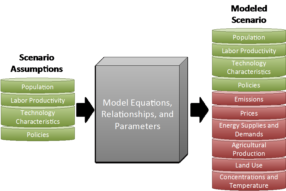
GCAM scenario assumptions and modelling outputs
Outcomes in GCAM depend strongly on the assumptions made for socioeconomic, techno-economic, and agronomic parameters. While many of these parameters matter for the outcomes from the model, some can be identified as the most relevant ones, given the purpose of GCAM in the framework of the PARIS REINFORCE project:
• Global and national GHG reduction targets • Global and national afforestation targets • Future demand scenarios for energy services and agricultural products • Future cost paths for renewable energy and CCS technologies
Parameters can be revised and updated in the framework of the PARIS REINFORCE project, following the feedback of local experts (stakeholder engagement), the comparative assessment with other modelling experiences, and the discussion with the partners (modellers).
Policy questions and SDGs
Key policies that can be addressed
One of GCAM’s uses is to explore the implications of different future policies. There are a number of types of policies that can be easily modelled in GCAM:
Emissions-related policies: There are three main policy approaches that can be applied in GCAM to reduce emissions of CO2 or other GHGs: carbon/GHG prices, emissions constraints, or climate constraints. In all cases, GCAM implements the policy approach by placing a price on emissions. This price then filters down through all systems in GCAM and alters production and demand. For example, a price on carbon would put a cost on emitting fossil fuels. This cost would then influence the cost of producing electricity from fossil-fired power plants that emit CO2, which would then influence their relative cost compared to other electricity generating technologies and increase the price of electricity. The increased price of electricity would then make its way to consumers that use electricity, decreasing its competitiveness relative to other fuels and leading to a decrease in electricity demand.
• Carbon or GHG prices: GCAM users can directly specify the price of carbon or GHG emissions. Given a carbon price, the resulting emissions will vary depending on other scenario drivers, such as population, GDP, resources, and technology. • Emissions constraints: GCAM users can specify the total amount of (CO2 or other GHG) emissions as well. GCAM will then calculate the price of carbon needed to reach the constraint in each period of the constraint. • Climate constraints: GCAM users can specify a climate variable (e.g. concentration or radiative forcing) target for a particular year. Users determine whether that target can be exceeded prior to the target year. GCAM will adjust carbon prices in order to find the least-cost path to reaching the target.
Emissions prices of different GHGs can be linked together for a multi-gas policy. Additionally, markets in GCAM can be set for any emission species (e.g., CH4-only market, NOx market, etc.). In addition to identifying emission prices as one measure of cost, GCAM employs the “deadweight loss” approach to measuring welfare loss from emissions mitigation efforts through carbon pricing.
Energy production policies: There are times when users would like to explore the implications of a constraint on production or a minimum production requirement. This capability allows GCAM users to model policies such as renewable portfolio standards and biofuels standards. Across sectors, these constraints must be applied as quantity constraints, but they can be applied as share constraints within individual sectors (e.g. fraction of electricity that comes from solar power). In implementing these policies, users can set either a lower bound or an upper bound. The model will solve for the tax (upper bound) or subsidy (lower bound) required to reach the given constraint.
Land use policies
• Protected Lands: With this policy, GCAM users can set aside a fraction of natural land, removing it from economic competition. This land cannot be converted to crops, pasture, or any other land type. This is similar to real-world policies such as reducing emissions from deforestation and forest degradation (REDD). • Valuing carbon in land: When applying a price on carbon through any of the emissions-related policy approaches, GCAM users can choose whether that price extends to land use change CO2 emissions. This policy is modelled as a subsidy to land-owners for holding carbon stocks as opposed to a price on the emissions themselves. • Bioenergy constraints: GCAM users can impose constraints on bioenergy within GCAM. Under such a policy, GCAM will calculate the tax or subsidy required to ensure that the constraint is met.
Key policies that can be addressed
GCAM does not automatically calculate the implications on non-climate SDGs of its least-cost energy system to meet prescribed climate or emissions constraints. However, it is possible to use its outputs and calculate the predictions for certain indicators framed in the SDG agenda.
| SDGs | GCAM |
|---|---|
| §2. Zero hunger (e.g., food prices, shortages) | Food prices by region |
| §3. Health (e.g., air-pollution related mortality) | Mortality due to air pollutants |
| §6. Clean water and sanitation (e.g., groundwater depletion) | Groundwater depletion by river basin |
| §7. Affordable and clean energy (e.g., traditional biomass use, %renewable energy) | Traditional biomass use and renewable energy penetration |
| §12: Responsible production & consumption (e.g., % recycled waste, embedded emissions) | Footprint impact of consumption |
| §15: Life on land (e.g., land use for forests, rate of land use change) | Land use for forests and rate of land use change |
Recent use cases
| Paper | Topic | Key Findings |
|---|---|---|
| (Huang et al., 2019) | Global agricultural green and blue water consumption under future climate and land use changes | Global crop green water consumption will increase by 12% in 2090s when compared with that in 1971–2000, and climate change will dominate over land use change in determining the trend of global crop green water consumption. However, expansion in global irrigated area will dominate the changing trend of global crop blue water consumption which increases 70% by 2090s, especially in regions with significant irrigated land expansion (e.g. northern Africa, central Asia, China, Mexico, the Middle East, Russia, southern Asia, and Argentina). Furthermore, global crop blue water dependence will increase under climate and land use changes, especially in arid regions. |
| (Markandya et al., 2018) | Health co-benefits from air pollution and mitigation costs of the Paris Agreement | The health co-benefits substantially outweighed the policy cost of achieving the 2°C target. The ratio of health co-benefit to mitigation cost ranged from 1.4 to 2.45, depending on the scenario. At the regional level, the costs of reducing GHG emissions could be compensated with the health co-benefits alone for China and India, whereas the proportion the co-benefits covered varied but could be substantial in the European Union (7–84%) and USA (10–41%), respectively. Finally, we found that the extra effort of trying to pursue the 1.5°C target instead of the 2°C target would generate a substantial net benefit in India (US$3.28–8.4 trillion) and China ($0.27–2.31 trillion). |
| (Fawcett et al., 2015) | Understanding what the INDCs collectively deliver in terms of reducing the probability of the highest levels of global mean surface temperature change and improving the odds of limiting temperature change to under 2°C relative to preindustrial levels | To limit warming to any level, CO2 emissions at the global level must ultimately be brought to zero. If emissions are not brought swiftly to zero beyond 2100, the chances of extreme temperature change after 2100 could be much higher and the chance of limiting warming to 2°C much lower. The Paris scenarios reduce probabilities of extreme warming and increase the probability of limiting global warming to 2°C this century. |
GCAM-China
Overview
The GCAM model was expanded to include greater spatial detail in the China region, referred to as GCAM-China. GCAM-China is built within the GCAM framework. Hence assumptions in GCAM-China are made in the same way as the rest of the model.
Key features of the GCAM-China model
In GCAM-China, the 31 Chinese provinces are included as explicit regions that operate within the global GCAM model. Energy transformation (electricity generation and refined liquids production) and end-use demands (buildings, transportation, and industry) are modelled at the individual province level, and inter-province trade of all energy goods is considered. For electricity trade between provinces, provinces are grouped into 6 grid regions. Whereby provinces within the same sub-region can trade freely within that sub-region, trade between regions may be limited. The following table shows an overview of features calibrated at the country, grid and province level. The model can generate pathways through to 2100 with 5 year time periods.
The more detailed province-level approach for China has advantages over the global version of GCAM, in terms of more detailed assumptions on socioeconomic and energy futures, resulting into potentially more realistic reference scenarios. Also, the higher geographical granularity as advantages for policy analysis and impacts of climate policies might differ strongly between provinces.
| Country level (China) | Grid-region level () | Province level |
|---|---|---|
| - Fossil fuel reserves, production and prices - Agriculture and land use - Biomass production and prices - International trade in energy commodities | - Final energy prices for electricity - Inter-regional electricity trade | - Renewable energy reserves and usage - Electricity production - Building energy end-use* - Industrial energy end-use - Transportation energy end-use - CCS reserves and usage |
| * Building energy end-use by state has a higher detail w.r.t. appliances use than in the global version | ||
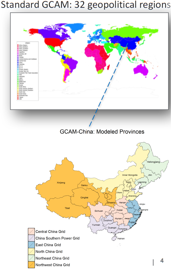
Geographical coverage of GCAM-China
Calibration of the model
The GCAM model is calibrated for its base year, 2010. For international and China-wide data, the same data sources are used for calibration as for the global model, which are predominantly IEA energy balances for energy production and consumption, and FAOSTAT balances for food demand and agriculture. For province- and grid-level data in China, national Chinese data sources have been used for calibration.
Key parameters
Outcomes in GCAM depend strongly on the assumptions made for socioeconomic, techno-economic, and agronomic parameters. Given the role that GCAM-China might play in the PARIS REINFORCE project, some input parameters will be most relevant for the model outcomes:
- Chinese national GHG reduction target and mitigation burden and other priorities by province
- Province-specific renewable and CCS resources
- nformation about under construction/planned/possible energy projects/infrastructures
- Future demand scenarios for energy services by province
Parameters can be revised and updated in the framework of the PARIS REINFORCE project, following the feedback of national-level experts (stakeholder engagement), the comparative assessment with other modelling experiences, and the discussion with the partners (modellers).
Recent publications using GCAM-China
| Ref | Title | Key findings |
|---|---|---|
| Yu et al. (2019) | CCUS in China's mitigation strategy: insights from integrated assessment modelling | The inclusion of new provincial CO2 storage cost curves gives a more detailed evaluation of where, in terms of geography and sector, and when CCUS deployment in China may take place. The results suggest that the scale of deployment varies depending on socioeconomic development pathways and the level of deployment of other low-carbon technologies. Across provinces and development pathways, early deployment of CCUS occurs within industrial and synthetic fuel production sectors, followed by increased deployment in the power sector by mid-century. Several provinces, such as Shandong, Inner Mongolia, Hebei, and Henan, emerge as particularly important in CCUS deployment, as a result of large CO2 point sources and storage availability. Results indicate that storage resource availability is unlikely to constrain CCUS deployment in most provinces through the end of the century. |
| Yu et al. (2014) | Scenarios of building energy demand for China with a detailed regional representation | The Cold and Hot Summer Cold Winter regions lead in total building energy use. The impact of climate change on heating energy use is more significant than that of cooling energy use in most climate regions. Both rural and urban households will experience fuel switch from fossil fuel to cleaner fuels. Commercial buildings will experience rapid growth in electrification and energy intensity. Improved understanding of Chinese buildings with climate change highlighted in his study help policymakers develop targeted policies and prioritise building energy efficiency measures. |
References
Yu, S., Horing, J., Liu, Q., Dahowski, R., Davidson, C., Edmonds, J., & Clarke, L. (2019). CCUS in China’s mitigation strategy: insights from integrated assessment modelling. International Journal of Greenhouse Gas Control, 84, 204-218.
Yu, S., Eom, J., Zhou, Y., Evans, M., & Clarke, L. (2014). Scenarios of building energy demand for China with a detailed regional representation. Energy, 67, 284-297.
GCAM-SOUSEI
Overview
GCAM-SOUSEI, like the GCAM model from which it is derived, is a multi-region global model, which includes Japan as a separate region. The level of energy system, agriculture and land use detail for the Japan region allows it to be used to study Japan’s national-level low-carbon pathways. In addition, GCAM-SOUSEI uses emission pathways that account for uncertainties in a number of climate-relevant parameters relating CO2 atmospheric concentrations to global temperature changes.
These emission pathways are obtained from a large set of experimental results with a climate model (Earth system model of intermediate complexity, or EMIC) covering a wider range of parameters and uncertainties than the original GCAM model, leading to a range of CO2 emissions being associated with each temperature change target.
The climate model in GCAM-SOUSEI emulates the Earth system, covering the range of values of physical and biogeochemical parameters indicated by multiple Earth System Models (ESMs), which are highly complex and detailed models used to analyse the global changes of the atmosphere, the land and the ocean (the original GCAM model includes a simple climate model called the Model for the Assessment of Greenhouse-gas Induced Climate Change, or MAGICC).
The emission pathways for allowable carbon emissions translate into lower total energy consumption, shift from high shares of fossil fuels to larger shares of renewables and nuclear energy, as well as the increase in CCS penetration. Also, larger amounts of bioenergy crops result in conversion of unmanaged land (pastures, arable land among others) into land for bioenergy crops.
Key features of the model
GCAM-SOUSEI combines detailed representations of the energy, land and agricultural systems with a climate model in the same way as for the main GCAM model. The model can generate pathways through to 2100 with 5 year time periods.
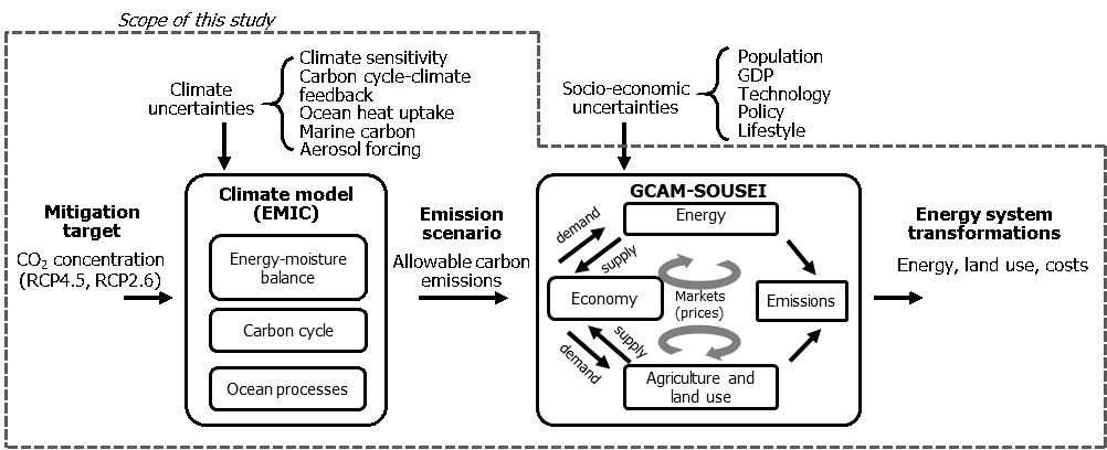
Modelling framework illustrating the main components and data flows in the EMIC climate model and GCAM-SOUSEI.
Recent publications using GCAM-SOUSEI
| Ref | Title | Key findings |
|---|---|---|
| Silva Herran et al. (2019) | Global energy system transformations in mitigation scenarios considering climate uncertainties | Even when climate uncertainties are reflected at different scales across energy supply components, achieving mitigation targets needs partial decarbonisation of supply, scaling up of carbon capture and storage (CCS), and decreased energy consumption. The effect of climate uncertainties was largest for coal without CCS (up to 100% in 2100 compared to the central scenario) and bioenergy with CCS (up to 23% in 2100 compared to the central scenario). Land for bioenergy feedstocks and the deployment of unmanaged lands for other purposes also had a considerable variation (10-20% in 2100). Compared to the uncertainty in socioeconomic factors quantified in IAMs, the variation induced by the climate uncertainties was small. |
References
Silva Herran, D., Tachiiri, K., & Matsumoto, K. I. (2019). Global energy system transformations in mitigation scenarios considering climate uncertainties. Applied energy, 243, 119-131.
GCAM-USA
Overview
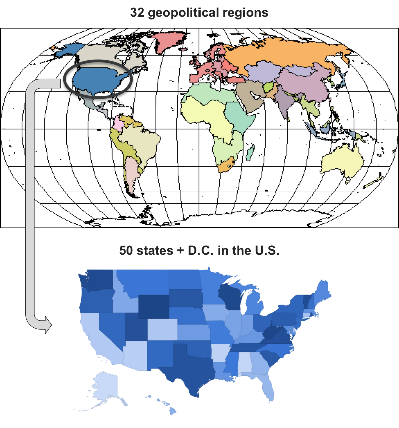
The GCAM model was expanded to include greater spatial detail in the USA region, referred to as GCAM-USA. GCAM-USA is built within the GCAM framework. Hence assumptions in GCAM-USA are made in the same way as the rest of the model.
In GCAM-USA, the 50 U.S. states plus the District of Columbia (hereafter, the 51 states) are included as explicit regions that operate within the global GCAM model. Energy transformation (electricity generation and refined liquids production) and end-use demands (buildings, transportation, and industry) are modelled at the individual state level, and inter-state trade of all energy goods is considered. For electricity trade between states, states are grouped into the 13 NEMS Electricity Market Module Regions (EIA 2010), plus Alaska and Hawaii. Whereby states within the same sub-region can trade freely within that sub-region, trade between regions may be limited. Also, prices for final energy commodities (except for biomass products) are calibrated per grid region, reflecting regional differences in energy prices. The following table shows an overview of features calibrated at the country, grid and state level.
Key features of the model
The more detailed state-level approach for the USA has advantages over the global GCAM model, in terms of more detailed assumptions on socioeconomic and energy futures, resulting into potentially more realistic reference scenarios. Also, the higher geographical granularity has advantages for policy analysis, as climate policies often vary by state in the USA, and impacts of climate policies might differ strongly between states.
| Country level (USA) | Grid-region level () | State level |
|---|---|---|
| - Fossil fuel reserves and production - Agriculture and land use - Biomass production and prices - International trade in energy commodities | - Final energy prices for electricity, liquids, gas and coal - CCS reserves and usage - Inter-regional electricity trade | - Renewable energy reserves and usage - Electricity production - Building energy end-use* - Industrial energy end-use - Transportation energy end-use |
| * Building energy end-use by state has a higher detail w.r.t. appliances use than in the global version | ||
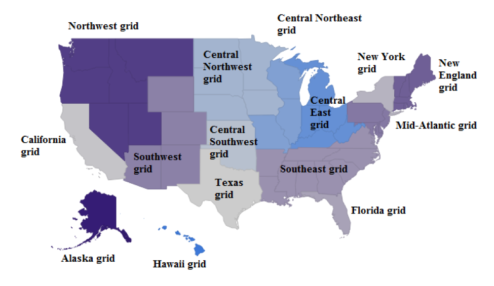
Geographical coverage of GCAM-USA
Calibration of the model
The GCAM model is calibrated for its base year, 2010. For international and USA-wide data, the same data sources are used for calibration as for the global model, which are predominantly IEA energy balances for energy production and consumption, and FAOSTAT balances for food demand and agriculture. For state- and grid-level data in the USA, the State Energy Data System from the EIA (2014) is used as the primary dataset. Socioeconomic data are calibrated for 2015 at the state-level, reflecting data from the U.S. Census Bureau.
Key parameters
Outcomes in GCAM depend strongly on the assumptions made for socioeconomic, techno-economic, and agronomic parameters. Given the role that GCAM-USA might play in the PARIS REINFORCE project, some input parameters will be most relevant for the model outcomes:
- US national/state-level GHG reduction targets and other priorities/plans
- State-specific renewable and CCS resources
- Information about under construction/planned/possible energy projects/infrastructures
- Future demand scenarios for energy services by state
Parameters can be revised and updated in the framework of the PARIS REINFORCE project, following the feedback of national-/state-level experts (stakeholder engagement), the comparative assessment with other modelling experiences, and the discussion with the partners (modellers).
Model presentation
Video
Slides
Download slides in pdfRecent publications using GCAM-USA
| Study | Focus | Key findings |
|---|---|---|
| Ou et al. (2018) | Estimating environmental co-benefits of U.S. low-carbon pathways using an integrated assessment model with state-level resolution | Air pollutant emissions, mortality costs attributable to particulate matter smaller than 2.5 µm in diameter, and energy-related water demands are evaluated for 50% and 80% CO2 reduction targets in 2050. The renewable low-carbon pathways require less water withdrawal and consumption than the nuclear and carbon capture pathways. However, the renewable low-carbon pathways modelled in this study produce higher particulate matter-related mortality costs due to greater use of biomass in residential heating. Environmental co-benefits differ among states because of factors such as existing technology stock, resource availability, and environmental and energy policies. |
| Iyer et al. (2017) | GCAM-USA Analysis of U.S. Electric Power Sector Transitions | The United States has developed a Mid-Century Strategy to reduce economy-wide greenhouse gas (GHG) emissions to 80% or more below 2005 levels by 2050. Achieving these reductions will entail a major transformation of the energy system, including the electric power sector. The scenarios in this study include substantial decarbonisation of the electric power sector, increased electrification of end-use sectors, and increase in the deployment of low- and zero-carbon technologies such as renewables, nuclear and carbon capture utilisation and storage. The results show that the degree to which the electric power sector will need to decarbonise depends on the nature of technological advances in the energy sector, and the degree to which end-use sectors electrify. |
| Feijoo et al. (2018) | The future of natural gas infrastructure development in the United states | Existing pipeline infrastructure in the U.S. is insufficient to satisfy the increasing demand for natural gas, and investments in pipeline capacity will be required. However, the geographic distribution of investments within the U.S. is heterogeneous and depends on the capacity of existing infrastructure as well as the magnitude of increase in demand. The results also illustrate the risks of under-utilisation of pipeline capacity, in particular, under a scenario characterised by long-term systemic transitions toward a low-carbon economy. More broadly, this study highlights the value of integrated approaches to facilitate informed decision-making. |
References
Feijoo, F., Iyer, G. C., Avraam, C., Siddiqui, S. A., Clarke, L. E., Sankaranarayanan, S., ... & Wise, M. A. (2018). The future of natural gas infrastructure development in the United States. Applied energy, 228, 149-166.
Iyer, G., Ledna, C., Clarke, L. E., McJeon, H., Edmonds, J., & Wise, M. (2017). GCAM-USA analysis of US electric power sector transitions. Richland, Washington: Pacific Northwest National Laboratory.
Ou, Y., Shi, W., Smith, S. J., Ledna, C. M., West, J. J., Nolte, C. G., & Loughlin, D. H. (2018). Estimating environmental co-benefits of US low-carbon pathways using an integrated assessment model with state-level resolution. Applied energy, 216, 482-493.
U.S. Energy Information Agency (EIA 2010) Annual Energy Outlook 2010 with projections to 2035. DOE/EIA-0383(2010).
