The Intertemporal Computable Equilibrium System (ICES) model
Short overview
ICES is a recursive-dynamic multi-regional Computable General Equilibrium (CGE) model developed to assess impacts of climate change on the economic system and to study mitigation and adaptation policies. The model’s general equilibrium structure allows for the analysis of market flows within a single economy and international flows with the rest of the world. This implies going beyond the “simple” quantification of direct costs, to offer an economic evaluation of second and higher-order effects within specific scenarios of climate change, climate policies and/or different trade and public-policy reforms in the vein of conventional CGE theory. The model is linked to the Aggregated Sustainable Development goal Index (ASDI) module that generates scenario and policy specific projections up to 2030 (2050) of selected SDG indicators allowing to assess the systemic implication of implementing a policy on countries’ sustainability.
Key features of the ICES model
Geographic coverage
The ICES model has worldwide coverage. In PARIS REINFORCE, the globe will be broken down into 45 countries or regions (see the table below).
| No. | Countries/regions | Detail | No. | Countries/regions | Detail | |
|---|---|---|---|---|---|---|
| 1 | Australia | Australia, Christmas Island, Cocos (Keeling) Islands, Heard Island and McDonald Islands, Norfolk Island | 24 | Germany | Germany | |
| 2 | NewZealand | NewZealand | 25 | Greece | Greece | |
| 3 | Japan | Japan | 26 | Italy | Italy | |
| 4 | South Korea | South Korea | 27 | Poland | Poland | |
| 5 | Bangladesh | Bangladesh | 28 | Spain | Spain | |
| 6 | China | China, Hong Kong, Taiwan | 29 | Sweden | Sweden | |
| 7 | India | India | 30 | UK | UK | |
| 8 | Indonesia | Indonesia | 31 | RoEU | Austria, Cyprus, Denmark, Estonia, Hungary, Ireland, Latvia, Lithuania, Malta, Portugal, Slovakia, Slovenia, Bulgaria, Croatia, Romania | |
| 9 | RoAsia | Mongolia, Democratic People's Republic of Korea, Macao, Cambodia, Lao PDR, Malaysia, Philippines, Singapore, Thailand, Viet Nam, Brunei Darussalam, Myanmar, Timor-Leste, Nepal, Pakistan, Sri Lanka, Afghanistan, Bhutan, Maldives | 32 | RoEurope | Switzerland, Norway, Svalbard and Jan Mayen Islands, Iceland, Liechtenstein, Albania, Belarus, Ukraine, Moldova, Andorra, Bosnia and Herzegovina, Faroe Islands, Gibraltar, Guernsey, Holy See ( Vatican City State), Isle of Man, Jersey, Republic of Macedonia, Monaco, Montenegro, San Marino, Serbia | |
| 10 | Canada | Canada | 33 | Russia | Russia | |
| 11 | USA | 34 | Turkey | Turkey | ||
| 12 | Mexico | Mexico | 35 | Egypt | Egypt | |
| 13 | Argentina | Argentina | 36 | RoMENA | ||
| 14 | Bolivia | Bolivia | 37 | Ethiopia | Ethiopia | |
| 15 | Brazil | Brazil | 38 | Ghana | Ghana | |
| 16 | Chile | Chile | 39 | Kenya | Kenya | |
| 17 | Peru | Peru | 40 | Mozambique | Mozambique | |
| 18 | Venezuela | Venezuela | 41 | Nigeria | Nigeria | |
| 19 | RoLACA | Colombia, Ecuador, Paraguay, Uruguay, Falkland Islands (Malvinas), French Guiana, Guyana, South Georgia and the South Sandwich Islands, Suriname, Costa Rica, Guatemala, Honduras, Nicaragua, Panama, El Salvador, Belize, Anguilla, Antigua and Barbuda, Aruba, Bahamas, Barbados, British Virgin Islands, Cayman Islands, Cuba, Dominica, Dominican Republic, Grenada, Haiti, Jamaica, Montserrat, Netherlands Antilles, Puerto Rico, Saint Kitts and Nevis, Saint Lucia, Saint Vincent and Grenadines, Trinidad and Tobago, Turks and Caicos Islands, Virgin Islands (US) | 42 | Uganda | Uganda | |
| 20 | Benelux | Belgium, Luxembourg, Netherlands | 43 | South Africa | South Africa | |
| 21 | Czech Republic | Czech Republic | 44 | RoAfrica | Cameroon, Côte d'Ivoire, Senegal, Benin, Burkina Faso, Cape Verde, Gambia, Guinea, Guinea-Bissau, Liberia, Mali, Mauritania, Niger, Saint Helena, Sierra Leone, Togo, Central African Republic, Chad, Congo, Equatorial Guinea, Gabon, Sao Tome and Principe, Angola, Democratic Republic of the Congo | |
| 22 | Finland | Finland | 45 | RoW | American Samoa, Cook Islands, Fiji, French Polynesia, Guam, Kiribati, Marshall Islands, Federated States of Micronesia, Nauru, New Caledonia, Niue, Northern Mariana Islands, Palau, Papua New Guinea, Pitcairn, Samoa, Solomon Islands, Tokelau, Tonga, Tuvalu, United States Minor Outlying Islands, Vanuatu, Wallis and Futuna Islands, Bermuda, Greenland, Saint Pierre and Miquelon, Kazakhstan, Kyrgyzstan, Tajikistan, Turkmenistan, Uzbekistan, Armenia, Azerbaijan, Georgia, Antarctica, Bouvet Island, British Indian Ocean Territory, French Southern Territories | |
| 23 | France | France |
Sectoral coverage
In each country, firms are grouped in 26 macro sectors that essentially comprise the economy (see the table below).
| Sectors | |||
|---|---|---|---|
| 1 | Agriculture | 14 | Hydro Electricity |
| 2 | Livestock | 15 | Nuclear Electricity |
| 3 | Processed Food | 16 | Other non-fossil Electricity |
| 4 | Forestry | 17 | Heavy Industries |
| 5 | Fishing | 18 | Light Industries |
| 6 | Other Mining | 19 | Transport |
| 7 | Coal | 20 | Water |
| 8 | Oil | 21 | R&D |
| 9 | Gas | 22 | Market Services |
| 10 | Oil Products | 24 | Health |
| 11 | Fossil Electricity | 25 | Education |
| 12 | Solar Electricity | 26 | Public Services |
| 13 | Wind Electricity | ||
Database
ICES is a computable model: all the model behavioural equations are connected to the GTAP 8 database (Narayanan, Badri, & McDougall, 2012), which collects national social accounting matrices from all over the world and provides a snapshot of all economic flows in the benchmark year (2007). All economic flows related to fuel-specific energy production and consumption derive from GTAP-Power database (Peters, 2016) and are merged to GTAP 8 database.
In order to perform a sustainability analysis, the GTAP database has been integrated with international statistics in order to single out the following sectors: Research and Development (R&D), Education, and Health. For the R&D sector, the indicator “R&D expenditure as percentage of GDP” from the World Development Indicators - WDI (World Bank 2016) and the “share of R&D financed by Government, Firms, Foreign Investment and Other National” from the OECD Main Science and Technology Indicators (OECD 2016) are used for attributing R&D to the different economic agents. A similar approach has been used for Education and Health sectors. Data on overall expenditure on health and education have been obtained from the WDI database (World Bank 2016).
The ICES database has been further extended following the model developments regarding the public actor (Delpiazzo, Parrado, & Standardi, 2017). In addition to government revenues and expenditures already included in GTAP 8 database, other monetary flows have been made explicit: international transactions among governments (foreign aid and grants) and transactions between the government and the private households (net social transfers, interest payment on public debt to residents), flows among governments and foreign private households (interest payment on public debt to non-residents), and public debt.
Emissions granularity
The model’s economic database is complemented with satellite databases on energy volumes (McDougall & Aguiar, 2008), CO2 and non‐CO2 emissions (Rose & Lee, 2008; Lee, 2008), which include nitrous oxide (N2O), methane (CH4), and three fluorinated gases (F‐gases). Both energy volumes and emissions have an endogenous dynamic in the models and evolve the former, according to energy sector production, and the latter, proportionally to energy combustion processes (CO2 emissions) and sectoral and household use of agricultural and energy commodities. GHG emissions do not include emissions from LULUCF (Land Use, Land Use Change and Forestry). The median trend of GHG emissions across IAM scenarios (IIASA database) is targeted given the pattern of energy prices and adjusting sector-specific efficiency in energy use.
Socioeconomic dimensions
The model is largely driven by the set of possible futures envisioned by the climate change community and known as Shared Socioeconomic Pathways (SSPs) (O’Neill, et al., 2017). These are five possible futures with different mitigation/adaptation challenges and are characterised by different evolutions of main socioeconomic variables. SSPs can be linked to Representative Concentration Pathways (RCPs) that envision the GHG emission evolution and forcing and temperature rise due to specific patterns of socioeconomic growth (Riahi, et al., 2017).
SSPs provide future patterns for population, working age population and GDP at country level; the trend of the first two variables is completely exogenous in our simulation. The GDP trend is instead a target to be met through a mix of country and sector-specific productivities that are exogenously set (primary factor and total factor productivity).
Calibration of the model
In our reference scenarios, the growth of GDP, population and employment reproduces historical trends up to 2014 (WDI 2016) and then mimics SSP growth rates (OECD projections). Population trend relies on the WDI database (World Bank 2018) up to 2014 and then follows SSP growth rates (IIASA-WiC projections). Employment trends rely on the WDI database (World Bank 2018) up to 2010, then consider IIASA-WiC projections of working age population and other specific assumption of SSP storylines: converging participation and unemployment rates in the long run to a structural level.
Mitigation/adaptation measures
The ICES model includes a climate policy module that allows designing mitigation policies through explicit or implicit carbon taxes internalising or correcting the external costs of polluting activities.
In the former case, carbon taxes are introduced into the model through specific ad valorem rates depending on the source of emissions. Carbon tax rates are calculated for each emitting source as the corresponding ratio between tax revenues and the total tax base. Then, this ad valorem tax is added to the supply price and determines the market price that households and firms finally face.
In the case of implicit carbon tax, regional emission limits can be imposed (quotas). Countries/regions can exchange emission rights starting from an initial allocation of permits in order to comply with the quota. The emission trade generates the optimal allocation of abatement and the emission price. In the ICES policy module, we can restrict emissions training to a set of countries, as in the case of EU-ETS, and combine it with direct carbon taxation in other countries, or allow for a global emissions trading system.
In the module, it is also possible to design mitigation scenarios curbing the carbon leakage effect (Border Tax Adjustments - BTA).
In each country/region revenues are collected by government that can use them to reduce public debt or increase government expenditure or rebate them to support household income (transfer), to subsidise specific firms or production factors (endowments or intermediates), and to support other countries (international transfer to specific countries or to an international fund, e.g. Green Climate Fund).
In addition to carbon taxation, ICES can implement other mitigation options such as subsidising clean energy production and its use (with direct effect on government deficit), imposing behavioural shifts on household and firm energy demand (without direct effect on government deficit), improving efficiency in energy use (with/without direct effect on government deficit), and applying the above described instruments and constraints to the agriculture, livestock and forestry sectors.
Economic rationale and model solution
The core structure of ICES derives from the GTAP-E model (Burniaux & Truong, 2002), which in turn is an extension of the standard GTAP model (Hertel, 1997). The General Equilibrium framework makes it possible to account for economic interactions of agents and markets within each country (production and consumption) and across countries (international trade). Within each country the economy is characterised by n industries, a representative household and the government. Industries are modelled as representative cost-minimising firms, taking input prices as given. In turn, output prices are given by average production costs. The production functions (see the figure below) are specified via a series of nested Constant Elasticity of Substitution (CES) functions. Primary factors—including natural resources, land, labour, and a capital-energy composite—constitute the Value Added Energy (QVAEN) nest, which is combined with intermediates (QF), in order to generate the output. Perfect complementarity is assumed between value added and intermediates. This implies the adoption of a Leontief production function. For sector i in region r, final supply (output)Yi,r, results from the following constrained production cost minimisation problem for the producer:
min PVAENi,rQ VAENi,r+PFi,rQFi,t
s.t.Yi,r=min[QVAENi,r,QFi,r]
where PVAEN and PF are prices of the related production factors.

ICES production tree
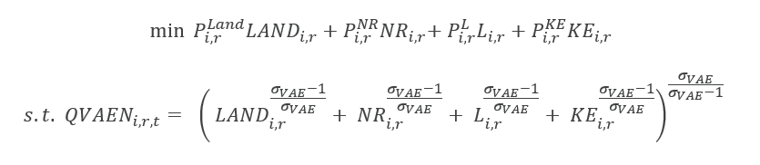
In the ICES production tree, the second nested level, on the left-hand side, represents the value added plus energy composite (QVAEN). This composite stems from a CES function that combines four primary factors: land (QLAND), natural resources (QNR), labour (QL) and the capital-energy bundle (QKE). Primary factor demand in turn derives from the first-order conditions of the following constrained cost minimisation problem for the representative firm:
In turn, the capital-energy bundle combines capital with a set of different energy inputs. In fact, energy inputs are not part of the intermediates, but are associated to capital in a specific composite. The energy bundle is modelled as an aggregate of electric and non-electric energy carriers. Electricity sector differentiates between intermittent and non-intermittent sources. Wind and solar, which are intermittent sources, are separated from non-intermittent sources: hydro, nuclear, fossil and other non-fossil electricity. Economic flows detailing production and consumption of energy relies on the GTAP-Power database (Peters, 2016).
The Non-Electric bundle is a composite of coal and energy from other fuels. The aggregate other fuels combine, in a series of subsequent nests, petroleum products with natural gas and crude oil. All elasticities regarding the inter-fuel substitution bundles are those from GTAP-E (Burniaux & Truong, 2002), while for the extended renewable electricity sectors we set those values considering different studies (Paltsev, et al., 2005; Bosetti, Carraro, Galeotti, Massetti, & Tavoni, 2006).
The demand of production factors (as well as that of consumption goods), can be met by either domestic or foreign commodities, which however are not perfectly substitutable according to the "Armington" assumption. In general, inputs grouped together are more easily substitutable among themselves than with other elements outside the nest. For example, the substitutability across imported goods is higher than that between imported and domestic goods. Analogously, composite energy inputs are more substitutable with capital than with other factors.
In the ICES model, as in GTAP, two industries are treated in a special way and are not related to any country, viz. international transport and international investment production. International transport is a world industry, which produces the transportation services associated with the movement of goods between origin and destination regions, thereby determining the cost margin between free-on-board (or f.o.b., before freight and insurance are added) and costs-insurance-freight (or c.i.f., inclusive of transportation margins) prices. Transport services are produced by means of factors submitted by all countries, in variable proportions. In a similar way, a hypothetical world bank collects savings from all regions and allocates investments in order to achieve equality in the absolute change of current rates of return.
The following figure describes the main sources and uses of regional income. In each region, a representative utility maximising household receives income, originated by the service value of national primary factors (natural resources, land, labour, and capital), that they own and sell to the firms. Capital and labour are perfectly mobile domestically but immobile internationally (investment is instead internationally mobile). Land and natural resources, on the other hand, are industry-specific and sluggish. Land is used only by the agriculture and livestock sectors, and competition for land is only among these two sectors; natural resources are of three types: forestry and fishing, fossil (coal, oil and gas), and other mining. Whether a sluggish endowment is used by more than one sector, its optimal allocation responds to the revenue maximisation of a household subject to a transformation frontier (Constant Elasticity of Transformation, or CET, formulation). Both land and natural resources are monetary aggregate variables in the base year, but price and quantity changes are distinguishable in simulation years.
The regional income is used to finance aggregate household consumption and savings.

Sources and uses of regional household income in ICES
Government income equals to the total tax revenues from both private households and productive sectors, a series of international transactions among governments (foreign aid and grants), and national government-private transfers (Delpiazzo, Parrado, & Standardi, 2017). Both the government and the private household consume and save a fraction of their income according to a Cobb-Douglas function. The government income not spent is saved, and the sum of public and private savings determines the regional disposable saving, which enters the Global Bank as in the core ICES model.
Both private and public sector consumption are addressed to all commodities produced by each firm/sector. Public consumption is split into a series of alternative consumption commodities according to a Cobb-Douglas specification. However, almost all public expenditure is concentrated in the specific sector of non-market services, including education, defence and health. Private consumption is analogously addressed towards alternative goods and services, including energy commodities that can be produced domestically or imported. The functional specification used at this level is the Constant Difference in Elasticities form: a non-homothetic function, which is used to account for possible differences in income elasticities for the various consumption goods2.
The recursive-dynamic feature is described in the following figure. Starting from the picture of the world economy in the benchmark year, by following socioeconomic (e.g. population, primary factors stocks and productivity) as well as policy-driven changes occurring in the economic system, agents adjust their decisions in terms of input mix (firms), consumption basket (households) and savings. The model finds a new general (worldwide and economy-wide) equilibrium in each period, while all periods are interconnected by the accumulation process of physical capital stock, net of its depreciation. Capital growth is standard along exogenous growth theory models and follows:
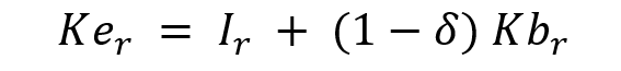
where Ker is the “end of period” capital Kbrstock, is the “beginning of period” capital stock, δ is capital depreciation and Iris endogenous investment. Once the model is solved at a given step t, the value of Ker is stored in an external file and used as the “beginning of period” capital stock of the subsequent step t+1.
The matching between savings and investments only holds at the world level; a fictitious world bank collects savings from all regions and allocates investments following the rule of highest capital returns.
As with capital, at each simulation step the government net deficit at the end of the period is stored in an external file and adds up to next year debt.

Recursive-dynamic feature of the ICES model
Policy questions and SDGs
Key policies that can be addressed
The model can be used to address a series of climate policy questions, orienting on overall sustainability. These include a deeper understanding of the feasibility of deep decarbonisation targets and related costs; of trade-offs between climate action, economic development and other societal targets; of possible economic evolution trajectories according to different climate policy scenarios; as well as of socioeconomic synergies and trade-offs between mitigation policies and activities oriented on sustainable development.
By looking into GHG emissions, including non-energy and agriculture emissions, the model can inter alia be used to determine national/regional compliance with (intended) nationally determined contributions, and assess gaps from equitable and sustainable emissions.
The ICES model can also be used to assess economy-wide implications of adaptation strategies (the term of comparison in this case is generally a scenario with climate change impacts), e.g. understanding the benefits of changing the crop mix in the case of impacts in agriculture or of building preventive protections in the case of sea level rise causing land loss, or delving into behavioural shifts or efficiency changes associated to climate change (e.g. higher cooling demand), which are imposed exogenously before their economy-wide implications are assessed).
Implications for other SDGs
The ASDI (Aggregated Sustainable Development goal Index) module aims at offering a comprehensive assessment of future sustainability up to 2030 (with the capacity to extend the analysis to 2050) based upon 27 indicators related to the 17 Sustainable Development Goals, under different socioeconomic and policy scenarios. ASDI module combines a modelling framework (ICES model) with an empirical one (regression approach based on historical data) to offer an internally-consistent set-up for analysing future patterns of sustainability indicators and their inter-linkages (see the figure below).

The ASDI module in ICES
Indicator selection is guided by the following requirements: relevance in measuring the SDG they refer to and connection with a specific quantitative SDG Target. Furthermore, ASDI indicators need to have good country coverage because the well-being assessment is worldwide and the comparability of the results of aggregation procedure requires excluding countries with missing values for at least one of ASDI indicators. ASDI indicators are at country level; the presence of a macro-economic model in our framework and the world coverage forces us to disregard more disaggregated indicators (gender, cohort, location-specific). Furthermore, the most stringent constraint in selecting ASDI indicators comes from the sustainability assessment: drawing the future path of SDG indicators depends on identifying their determinants (empirical analysis on the historical data and evidence from the literature), and, at the same time, depicting the future evolution of these determinants using the ICES model. The lack of any empirical evidence connecting an SDG indicator with one or more endogenous variable in our model determined its exclusion from ICES set of indicators. The following table lists all ASDI indicators, except for those referring to climate action (SDG 13).
| SDG | ASDI Indicator | Modelling Behaviour |
|---|---|---|
| SDG1 | Poverty headcount ratio at $1.90 a day (PPP2011) (% of population) | GDPPPP per capita and Palma ratio (regression) |
| SDG2 | Prevalence of undernourishment (% of population) | GDPPPP per capita, squared GDPPPP per capita, Palma ratio, urban population share, agricultural production per capita (regression) |
| SDG3a | Physician density (per 1000 population) | Health expenditure per capita and private heath expenditure share (regression) |
| SDG3b | Healthy Life Expectancy (HALE) at birth (years) | Physician density, education expenditure per capita, electricity access, undernourishment prevalence, urban population share (regression) |
| SDG4 | Youth literacy rate (% of population 15-24 years) | Public education expenditure per capita, urban population share (regression) |
| SDG6 | Annual freshwater withdrawals, total (% of internal renewable water) | Domestic demand of water by agents: households, industry, agriculture (endogenous) |
| SDG7a | Access to electricity (% of total population) | GDPPPP per capita, GDPPPP per capita squared, electricity output per capita, urbanisation and Palma ratio (regression) |
| SDG7b | Renewable electricity (% in total electricity output) | Supply of Electricity from Renewables and Total Electricity (endogenous) |
| SDG7c | Primary energy intensity (MJ / $PPP2011) | Total Primary Energy Supply and Real GDP (endogenous) |
| SDG8a | GDP per capita growth (%) | GDP (endogenous) and Population (exogenous) |
| SDG8b | GDP per person employed ($PPP2011) | GDP (endogenous) and Employed Population (exogenous) |
| SDG8c | Employment-to-population ratio (%) | Exogenous |
| SDG9a | Manufacturing value added (% of GDP) | Value Added in Manufacturing and GDP (endogenous) |
| SDG9b | Total energy and industry-related GHG emissions over sectoral value added (t of CO2e / $PPP2011) | Industrial Emissions and Value Added in the Industrial sector (endogenous) |
| SDG9c | Research and development (R&D) expenditure (% of GDP) | R&D Value Added and GDP (endogenous) |
| SDG10 | Palma ratio | Sectoral VA, public education expenditure per capita, unemployment and corruption control (regression) |
| SDG11 | CO2 intensity of residential and transport sectors (t of CO2 / t of oil equivalent energy use) | Demand of Fossil Fuels and Emissions in Residential and Transport sectors (endogenous) |
| SDG12 | Material productivity ($PPP2011/ kg) | Material (mining) Use in Heavy Industry sector and GDP (endogenous) |
| SDG14 | Marine protected areas (% of territorial waters) | Exogenous |
| SDG15a | Terrestrial protected areas (% of total land area) | Exogenous |
| SDG15b | Forest area (% of land area) | Land use in the Forestry sector (endogenous) |
| SDG15c | Endangered and vulnerable (animals and plants) species (% of total species) | Exogenous |
| SDG16 | Corruption Perception Index | Exogenous |
| SDG17 | General government gross debt (% of GDP) | GDP and government debt (endogenous) |
Among ASDI indicators, sixteen are computed using model results, seven require regression analyses to be linked to them (SDG1, SDG2, SDG3a, SDG3b, SDG4, SDG7a, SDG10), and the remaining four are kept constant at historical levels (SDG14, SDG15a, SDG15c, SDG16). The collection of historical data of indicators relies on several international databases (World Development Indicators (World Bank, 2018), the UN database (United Nations, 2018), and World Income Inequality Database (WIID3.4) (United Nations, 2017b), and covers all available countries for the period 1990-2015.
Historical data are used for initialising indicators in the base year of the model (2007) and for estimating the basic relationships between the model’s variables and indicators in the regression analysis phase. The ASDI module computes the values of the SDG indicators up to 2030 (2050) using the output of the ICES model. For the indicators not directly generated by the model, the estimated relationships from historical data with the regression analysis are used in an out-of-sample estimation procedure and combined with output variables of the model (main drivers are listed in the following table). In order to derive SDG-specific indices (simple average of the underlying indicators) and the ASDI, ASDI indicator values are normalised, using a benchmarking procedure that identifies sustainable and unsustainable thresholds, and then aggregated.
Recent use cases
| Paper | Topic | Key findings |
|---|---|---|
| Campagnolo & Davide, 2019 | Potential synergies and trade-offs between emission reduction policies and sustainable development objectives (ex-ante assessment of the impacts of the NDCs on the SDGs of poverty eradication and reduced income inequality | Our study finds that a full implementation of the emission reduction contributions, stated in the NDCs, is projected to slow down the effort to reduce poverty by 2030 (+4.2% of the population below the poverty line compared to the baseline scenario), especially in countries that have proposed relatively more stringent mitigation targets and suffer higher policy costs. Conversely, the impact of climate policy on inequality shows opposite sign but remains very limited. If financial support for mitigation action in developing countries is provided through an international climate fund, the prevalence of poverty will be slightly reduced at the aggregate level, but the country-specific effect depends on the relative size of funds flowing to beneficiary countries and on their economic structure. |
| Campagnolo & Ciferri, 2018 | Investigation of the current well-being and the future sustainability of Italy | We provide evidence that in a scenario business-as-usual, Italy will not improve significantly its level of well-being. However, with a set of policies specifically targeted in 2030, the Italian sustainability would increase remarkably especially if all policies were implemented simultaneously. |
| Campagnolo, et al., 2016 | Examination of recent developments in international climate policy, considering different levels of cooperation that may arise in light of the outcomes of the Conference of the Parties held in Doha | We find that the environmental component of sustainability improves at the regional and world level thanks to the implementation of climate policies. Overall sustainability increases in all scenarios since the economic and social components are affected negatively yet marginally. This analysis does not include explicitly climate change damages and this may lead to underestimating the benefits of policy actions. If the USA, Canada, Japan and Russia did not contribute to mitigating emissions, sustainability in these countries would decrease and the overall effectiveness of climate policy in enhancing global sustainability would be offset. |
| Virdis, Gaeta, De Cian, & Parrado, 2015 | Alternative pathways to achieve deep decarbonisation in Italy | The DDPs require considerable effort in terms of low-carbon resources and technologies. They also require considerable effort in economic terms. The cost changes, compared to a Reference Scenario, are significant: up to 30% higher cumulative net costs over the period 2010-2050. In particular, the emphasis switches from fossil fuel costs and operating costs towards investments in power generation capacity and more efficient technologies and processes |
| Raitzer, et al., 2015 | Examination of potential regimes for regulating global GHG emissions through 2050 in Indonesia, Malaysia, the Philippines, Thailand, and Vietnam | The analysis affirms that a global climate arrangement that keeps mean warming below 2°C is in the economic interest of the region. Although the policy costs for such stabilisation during initial decades are not trivial, net benefits are found to far exceed net costs. The resource requirements are also not insurmountable, as costs are a smaller share of GDP than what the region has spent in recent years on fossil fuel subsidies. Moreover, the study finds that policy costs to achieve stabilisation sharply increase if actions to reduce emissions are delayed |
References
O’Neill, B. C., Kriegler, E., Ebi, K. L., Kemp-Benedict, E., Riahi, K., Rothman, D. S., ... & Levy, M. (2017). The roads ahead: Narratives for shared socioeconomic pathways describing world futures in the 21st century. Global Environmental Change, 42, 169-180.
Riahi, K., Van Vuuren, D. P., Kriegler, E., Edmonds, J., O’neill, B. C., Fujimori, S., ... & Lutz, W. (2017). The shared socioeconomic pathways and their energy, land use, and greenhouse gas emissions implications: an overview. Global Environmental Change, 42, 153-168.
Paltsev, S., Reilly, J. M., Jacoby, H. D., Eckaus, R. S., McFarland, J. R., Sarofim, M. C., ... & Babiker, M. H. (2005). The MIT emissions prediction and policy analysis (EPPA) model: version 4. MIT Joint Program on the Science and Policy of Global Change.
Bosetti, V., Carraro, C., Galeotti, M., Massetti, E., & Tavoni, M. (2006). WITCH a world induced technical change hybrid model. The Energy Journal, 13-37.
Campagnolo, L., Carraro, C., Davide, M., Eboli, F., Lanzi, E., & Parrado, R. (2016). Can climate policy enhance sustainability?. Climatic change, 137(3-4), 639-653.
Raitzer, D. A., Bosello, F., Tavoni, M., Orecchia, C., Marangoni, G., & Samson, J. N. G. (2015). SouthEast Asia and the economics of global climate stabilization. Asian Development Bank.
